In the previous post, I mentioned that there are two more major aspects to discuss in designing ports:
- Modes Solvers (Eigenmode Solvers, Actually).
- How to place and design the ports.
I’ll start from the first for two reasons: One, is that it has direct implications over the second. Two, it is what I have been currently working on, in my personal projects.
This post only discusses Modal Solvers (as they are called in HFSS), naturally. Terminal based ports, e.g. discrete ports and the Driven Terminal solver in HFSS (that I am very ambivalent about) are more worth discussing in the last subject, correct port placement and design.
Introduction to Port Solvers
So what does a port-solver do? It starts off by taking a lateral cut of the geometry, for example, in a Microstrip line
the cut looks something like this

Then the a mesh needs to be applied, so the problem can be made discrete, as customary in Finite Element Method (FEM) solvers.

Now the eigenmode solver can be applied!
This is an excellent spot to give some credits, all around.
- The demonstrations I am making here are part of my own project, residing here, in my github repo.
- The project relies heavily on the “geometry” toolbox, existing in GNU-Octave.
- The meshing library used here is MESH2D, written by the wonderful Darren Engwirda. Although I have been promising (mostly myself) that this project will be done for more than two years, I give him the proper respect for sitting and writing this stuff down, while actually giving me support along the way.
Having been through all that, two-dimensional eigenmode solvers are a bit exhausting mathematically. So for the sake of example I will make the demonstration using a 1D port mode variation. If you do want to read about 2D Eigenmode solvers, I always recommend “The Finite Element Method in Electromagnetics”, by Prof. Jianming Jin.
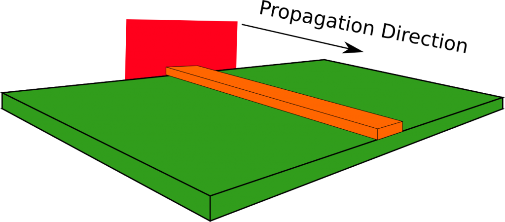
So let’s give some background on the 1D problem. For example, say we want to solve a problem that is Z-Infinite (I know it doesn’t exist, but it does demonstrate, in good approximation, a lot of problems) and single polarized. For instance, let’s take this Horn antenna, designed with my own 2D modeler.

The boundary conditions are radiating boundary conditions, and the Waveguide leading to the Antenna is infused by the red slab, denoting the port (PEC shielded). Again, meshing is applied to the model:

Before doing some actual mathematical work, the mesh segments along the port (denoted in the bright red line in the picture above) must be marked by their proper material.

So now we can start discussing the math behind it all. Most of the background data I based on “The Finite Element Method in Electromagnetics”, 1st edition, Chapters 3 and 7.
Math From Here To the Next Section, Skip If You Want
Let’s begin by formulating the wave equations for the two possible polarizations, in two dimensions:
![\mathbf{TE}_z\,:\,\left[{\frac{\partial}{\partial x}\left({\frac{1}{\epsilon_r}\frac{\partial}{\partial x}\bullet}\right)+\frac{\partial}{\partial y}\left({\frac{1}{\epsilon_r}\frac{\partial}{\partial y}\bullet}\right)+k_0^2\mu_r\bullet}\right]H_z=0](https://s0.wp.com/latex.php?latex=%5Cmathbf%7BTE%7D_z%5C%2C%3A%5C%2C%5Cleft%5B%7B%5Cfrac%7B%5Cpartial%7D%7B%5Cpartial+x%7D%5Cleft%28%7B%5Cfrac%7B1%7D%7B%5Cepsilon_r%7D%5Cfrac%7B%5Cpartial%7D%7B%5Cpartial+x%7D%5Cbullet%7D%5Cright%29%2B%5Cfrac%7B%5Cpartial%7D%7B%5Cpartial+y%7D%5Cleft%28%7B%5Cfrac%7B1%7D%7B%5Cepsilon_r%7D%5Cfrac%7B%5Cpartial%7D%7B%5Cpartial+y%7D%5Cbullet%7D%5Cright%29%2Bk_0%5E2%5Cmu_r%5Cbullet%7D%5Cright%5DH_z%3D0&bg=ffffff&fg=000000&s=2 "\mathbf{TE}_z\,:\,\left[{\frac{\partial}{\partial x}\left({\frac{1}{\epsilon_r}\frac{\partial}{\partial x}\bullet}\right)+\frac{\partial}{\partial y}\left({\frac{1}{\epsilon_r}\frac{\partial}{\partial y}\bullet}\right)+k_0^2\mu_r\bullet}\right]H_z=0")
![\mathbf{TM}_z\,:\,\left[{\frac{\partial}{\partial x}\left({\frac{1}{\mu_r}\frac{\partial}{\partial x}\bullet}\right)+\frac{\partial}{\partial y}\left({\frac{1}{\mu_r}\frac{\partial}{\partial y}\bullet}\right)+k_0^2\epsilon_r\bullet}\right]E_z=0](https://s0.wp.com/latex.php?latex=%5Cmathbf%7BTM%7D_z%5C%2C%3A%5C%2C%5Cleft%5B%7B%5Cfrac%7B%5Cpartial%7D%7B%5Cpartial+x%7D%5Cleft%28%7B%5Cfrac%7B1%7D%7B%5Cmu_r%7D%5Cfrac%7B%5Cpartial%7D%7B%5Cpartial+x%7D%5Cbullet%7D%5Cright%29%2B%5Cfrac%7B%5Cpartial%7D%7B%5Cpartial+y%7D%5Cleft%28%7B%5Cfrac%7B1%7D%7B%5Cmu_r%7D%5Cfrac%7B%5Cpartial%7D%7B%5Cpartial+y%7D%5Cbullet%7D%5Cright%29%2Bk_0%5E2%5Cepsilon_r%5Cbullet%7D%5Cright%5DE_z%3D0&bg=ffffff&fg=000000&s=2 "\mathbf{TM}_z\,:\,\left[{\frac{\partial}{\partial x}\left({\frac{1}{\mu_r}\frac{\partial}{\partial x}\bullet}\right)+\frac{\partial}{\partial y}\left({\frac{1}{\mu_r}\frac{\partial}{\partial y}\bullet}\right)+k_0^2\epsilon_r\bullet}\right]E_z=0")
Now since the ports are always planar, we can always find a rotation transformation, e.g.

that transforms the previous wave equations to
![\mathbf{TE}_z\,:\,\left[{\frac{\partial}{\partial \xi}\left({\frac{1}{\epsilon_r}\frac{\partial}{\partial \xi}\bullet}\right) + \frac{\partial}{\partial \zeta}\left({\frac{1}{\epsilon_r}\frac{\partial}{\partial \zeta}\bullet}\right) + k_0^2\mu_r\bullet}\right]H_z=0](https://s0.wp.com/latex.php?latex=%5Cmathbf%7BTE%7D_z%5C%2C%3A%5C%2C%5Cleft%5B%7B%5Cfrac%7B%5Cpartial%7D%7B%5Cpartial+%5Cxi%7D%5Cleft%28%7B%5Cfrac%7B1%7D%7B%5Cepsilon_r%7D%5Cfrac%7B%5Cpartial%7D%7B%5Cpartial+%5Cxi%7D%5Cbullet%7D%5Cright%29+%2B+%5Cfrac%7B%5Cpartial%7D%7B%5Cpartial+%5Czeta%7D%5Cleft%28%7B%5Cfrac%7B1%7D%7B%5Cepsilon_r%7D%5Cfrac%7B%5Cpartial%7D%7B%5Cpartial+%5Czeta%7D%5Cbullet%7D%5Cright%29+%2B+k_0%5E2%5Cmu_r%5Cbullet%7D%5Cright%5DH_z%3D0&bg=ffffff&fg=000000&s=2 "\mathbf{TE}_z\,:\,\left[{\frac{\partial}{\partial \xi}\left({\frac{1}{\epsilon_r}\frac{\partial}{\partial \xi}\bullet}\right) + \frac{\partial}{\partial \zeta}\left({\frac{1}{\epsilon_r}\frac{\partial}{\partial \zeta}\bullet}\right) + k_0^2\mu_r\bullet}\right]H_z=0")
![\mathbf{TM}_z\,:\,\left[{\frac{\partial}{\partial \xi}\left({\frac{1}{\mu_r}\frac{\partial}{\partial \xi}\bullet}\right)+\frac{\partial}{\partial \zeta}\left({\frac{1}{\mu_r}\frac{\partial}{\partial \zeta}\bullet}\right) + k_0^2\epsilon_r\bullet}\right]E_z = 0](https://s0.wp.com/latex.php?latex=%5Cmathbf%7BTM%7D_z%5C%2C%3A%5C%2C%5Cleft%5B%7B%5Cfrac%7B%5Cpartial%7D%7B%5Cpartial+%5Cxi%7D%5Cleft%28%7B%5Cfrac%7B1%7D%7B%5Cmu_r%7D%5Cfrac%7B%5Cpartial%7D%7B%5Cpartial+%5Cxi%7D%5Cbullet%7D%5Cright%29%2B%5Cfrac%7B%5Cpartial%7D%7B%5Cpartial+%5Czeta%7D%5Cleft%28%7B%5Cfrac%7B1%7D%7B%5Cmu_r%7D%5Cfrac%7B%5Cpartial%7D%7B%5Cpartial+%5Czeta%7D%5Cbullet%7D%5Cright%29+%2B+k_0%5E2%5Cepsilon_r%5Cbullet%7D%5Cright%5DE_z+%3D+0+&bg=ffffff&fg=000000&s=2 "\mathbf{TM}_z\,:\,\left[{\frac{\partial}{\partial \xi}\left({\frac{1}{\mu_r}\frac{\partial}{\partial \xi}\bullet}\right)+\frac{\partial}{\partial \zeta}\left({\frac{1}{\mu_r}\frac{\partial}{\partial \zeta}\bullet}\right) + k_0^2\epsilon_r\bullet}\right]E_z = 0")
Now, the solution for a forward propagating waveguide mode customary takes the form
 = u(\xi)e^{-ik_\zeta\zeta}")
 = u(\xi)e^{-ik_\zeta\zeta}")
where 

![\mathbf{TE}_z\,:\,\left[{\frac{\partial}{\partial \xi}\left({\frac{1}{\epsilon_r}\frac{\partial}{\partial \xi}\bullet}\right) + k_\xi^2\mu_r\bullet}\right]u=0](https://s0.wp.com/latex.php?latex=%5Cmathbf%7BTE%7D_z%5C%2C%3A%5C%2C%5Cleft%5B%7B%5Cfrac%7B%5Cpartial%7D%7B%5Cpartial+%5Cxi%7D%5Cleft%28%7B%5Cfrac%7B1%7D%7B%5Cepsilon_r%7D%5Cfrac%7B%5Cpartial%7D%7B%5Cpartial+%5Cxi%7D%5Cbullet%7D%5Cright%29++%2B+k_%5Cxi%5E2%5Cmu_r%5Cbullet%7D%5Cright%5Du%3D0&bg=ffffff&fg=000000&s=2 "\mathbf{TE}_z\,:\,\left[{\frac{\partial}{\partial \xi}\left({\frac{1}{\epsilon_r}\frac{\partial}{\partial \xi}\bullet}\right) + k_\xi^2\mu_r\bullet}\right]u=0")
![\mathbf{TM}_z\,:\,\left[{\frac{\partial}{\partial \xi}\left({\frac{1}{\mu_r}\frac{\partial}{\partial \xi}\bullet}\right) + k_\xi^2\epsilon_r\bullet}\right]u=0](https://s0.wp.com/latex.php?latex=%5Cmathbf%7BTM%7D_z%5C%2C%3A%5C%2C%5Cleft%5B%7B%5Cfrac%7B%5Cpartial%7D%7B%5Cpartial+%5Cxi%7D%5Cleft%28%7B%5Cfrac%7B1%7D%7B%5Cmu_r%7D%5Cfrac%7B%5Cpartial%7D%7B%5Cpartial+%5Cxi%7D%5Cbullet%7D%5Cright%29+%2B+k_%5Cxi%5E2%5Cepsilon_r%5Cbullet%7D%5Cright%5Du%3D0&bg=ffffff&fg=000000&s=2 "\mathbf{TM}_z\,:\,\left[{\frac{\partial}{\partial \xi}\left({\frac{1}{\mu_r}\frac{\partial}{\partial \xi}\bullet}\right) + k_\xi^2\epsilon_r\bullet}\right]u=0")
where
 = u(\xi)e^{-ik_\zeta\zeta}")
 = u(\xi)e^{-ik_\zeta\zeta}")
Now, to formulate as an FEM problem, let’s define the 1D Sturm–Liouville operator
 + \lambda\beta\phi = f")
while in the equations presented above,


As usual, in FEM formulations (if you are not familiar with these, don’t worry), the domain is disected into segments, as shown above. each segment is denoted with the index counter e. In this case, the basis functions chosen are 1st order functions, such that for each segment e applies
 = \sum\limits_{j=1}^{2}N_j^e(\xi)\phi_j^e\,;\,N_1^e(\xi) = \frac{\xi_2^e - \xi}{l_e},\,N_2^e(\xi) = \frac{\xi - \xi_1^e}{l_e}")
where 


where A and B are assembled from the subsets

that are assembled by

There is another difference between the TE and TM cases, that the boundary condition

needs to be imposed in TM. I am hardly getting into any implementation notes regarding FEM, so that won’t be elaborated here, as well. The important thing to remember here, is that the number of eigenmodes calculated is the same as the number of Non-metallic nodes. As far as this port goes, it will be 5 in the TE case and 3 in the TM case.
Once the mode is known, applying it to the 2D problem as a port is simple enough, by applying a boundary condition of the style
 - ik_\zeta u_0(\xi) e^{-ik_\zeta \zeta},")
where u0 is the mode chosen.
Now Pretty Pictures Again
So looking at the formulation above, we can say that the eigenvalues are related to the cutoff frequency, by

Whereas the eigenvectors represent the field distribution across the port. So let’s calculate them and see what happens!
Important notes:
- This was done without any port refinement (yet).
- The maximal number of modes was calculated. This isn’t always wise, especially not in this degenerated 1D case.
So let’s talk about the results we got.

Okay, so in the TE modes, the fundamental mode is actually a TEM mode. That makes sense, since this is a Z infinite problem and this is actually a 2 conductor waveguide.
Then next mode occurs about when the waveguide is at half wavelength, which makes sense. This also implies that this was a poor choice of waveguide dimensions, if I intend to simulate at about 30 GHz. This happens in both TE and TM cases, as can be seen below. The next mode mode is at about double that, at full wavelength, with two peaks. The amplitudes between the cases are opposite, as the B.C. are imposed on the TM case.
What happens after that is a mystery. We get a periodic recurrence of these modes. Does this make any sense? Probably not. I mean, these modes do exist, but they certainly don’t have these insane cutoffs. I will leave this to myself as homework, and hopefully I’ll have an answer some day.

I always find it crazy that this kind of heap of information, can be found at as little as 6 segments. The approximation here is bad, meshing is hardly sufficient, but still, we get reasonable data! Math wins, again.
So hopefully one day I’ll finish the 2D solver, so you can use publicly as a mode calculator. Otherwise, that’s it. You saw a bit about how mode solvers work, and feel free to contact me with any questions.