This post concerns a much more simplified version of the previous one. Last time we dealt with an arbitrary length line, with an unknown characteristic impedance. For that matter, a double length line de-embedding structure was suggested. In this post, we will deal with a more harried version of the process. Namely, when the designer didn’t print a specifically made de-embedding structure, but still needs to change the calibration plane. For that, most VNAs (or ENAs, or PNAs…) have a port extension function.
The port extension function, however, has some noticeable deficiencies. In this post we will discuss some of them. A quick review: In general, scattering matrix of an arbitrary impedance transmission line is
 \sinh \gamma l}\begin{bmatrix}\left({\frac{Z_c}{Z_0} - \frac{Z_0}{Z_c}}\right) \sinh \gamma l & 2 \ 2 & \left({\frac{Z_c}{Z_0} - \frac{Z_0}{Z_c}}\right) \sinh \gamma l \end{bmatrix}")
where
 \sinh \gamma l")
This is similar to the formulation given in the previous post, with
")
In order to de-embed the reflection at the load, we obtain the formula
![\Gamma_L = \frac{\Gamma_m - \frac{1}{\Delta_l}\left({1+\zeta - \frac{1}{1+\zeta}}\right)\sinh \gamma l}{\frac{1}{\Delta_l}\left({1+\zeta - \frac{1}{1+\zeta}}\right)\sinh \gamma l\left[{\Gamma_m - \frac{1}{\Delta_l}\left({1+\zeta - \frac{1}{1+\zeta}}\right)\sinh \gamma l} \right] + \frac{4}{\Delta_l^2}}](https://s0.wp.com/latex.php?latex=%5CGamma_L+%3D+%5Cfrac%7B%5CGamma_m+-+%5Cfrac%7B1%7D%7B%5CDelta_l%7D%5Cleft%28%7B1%2B%5Czeta+-+%5Cfrac%7B1%7D%7B1%2B%5Czeta%7D%7D%5Cright%29%5Csinh+%5Cgamma+l%7D%7B%5Cfrac%7B1%7D%7B%5CDelta_l%7D%5Cleft%28%7B1%2B%5Czeta+-+%5Cfrac%7B1%7D%7B1%2B%5Czeta%7D%7D%5Cright%29%5Csinh+%5Cgamma+l%5Cleft%5B%7B%5CGamma_m+-+%5Cfrac%7B1%7D%7B%5CDelta_l%7D%5Cleft%28%7B1%2B%5Czeta+-+%5Cfrac%7B1%7D%7B1%2B%5Czeta%7D%7D%5Cright%29%5Csinh+%5Cgamma+l%7D+%5Cright%5D+%2B+%5Cfrac%7B4%7D%7B%5CDelta_l%5E2%7D%7D&bg=ffffff&fg=000000&s=3 "\Gamma_L = \frac{\Gamma_m - \frac{1}{\Delta_l}\left({1+\zeta - \frac{1}{1+\zeta}}\right)\sinh \gamma l}{\frac{1}{\Delta_l}\left({1+\zeta - \frac{1}{1+\zeta}}\right)\sinh \gamma l\left[{\Gamma_m - \frac{1}{\Delta_l}\left({1+\zeta - \frac{1}{1+\zeta}}\right)\sinh \gamma l} \right] + \frac{4}{\Delta_l^2}}")
While performing port-extension de-embedding, a transmission line of similar length to the actual one is used. There reference load is either a short circuit or open circuit. These are a lot of words that mean the following: You can solder a short or disconnect the load, thus obtaining a short/open circuit load.
The Setup
In this example, we have a Device Under Test (DUT), an interface point and the previously mentioned unknown transmission line length. In the picture below, the DUT is a 2.4 GHz antenna. A 0 Ohm resistor is separating between the T-Line and the DUT. This resistor can be disconnected, thus allowing an open-load port extension.

Standard Port Extension
In this post I will demonstrate only the Open-Circuit (OC) case, but the development for the Short-Circuit one is very similar. The reflection coefficient of an OC load is 1. Substituting in the de-embedding formula, we obtain
![1 = \frac{\Gamma_m - \frac{1}{\Delta_l}\left({1+\zeta - \frac{1}{1+\zeta}}\right)\sinh \gamma l}{\frac{1}{\Delta_l}\left({1+\zeta - \frac{1}{1+\zeta}}\right)\sinh \gamma l\left[{\Gamma_m - \frac{1}{\Delta_l}\left({1+\zeta - \frac{1}{1+\zeta}}\right)\sinh \gamma l} \right] + \frac{4}{\Delta_l^2}}](https://s0.wp.com/latex.php?latex=1+%3D+%5Cfrac%7B%5CGamma_m+-+%5Cfrac%7B1%7D%7B%5CDelta_l%7D%5Cleft%28%7B1%2B%5Czeta+-+%5Cfrac%7B1%7D%7B1%2B%5Czeta%7D%7D%5Cright%29%5Csinh+%5Cgamma+l%7D%7B%5Cfrac%7B1%7D%7B%5CDelta_l%7D%5Cleft%28%7B1%2B%5Czeta+-+%5Cfrac%7B1%7D%7B1%2B%5Czeta%7D%7D%5Cright%29%5Csinh+%5Cgamma+l%5Cleft%5B%7B%5CGamma_m+-+%5Cfrac%7B1%7D%7B%5CDelta_l%7D%5Cleft%28%7B1%2B%5Czeta+-+%5Cfrac%7B1%7D%7B1%2B%5Czeta%7D%7D%5Cright%29%5Csinh+%5Cgamma+l%7D+%5Cright%5D+%2B+%5Cfrac%7B4%7D%7B%5CDelta_l%5E2%7D%7D&bg=ffffff&fg=000000&s=3 "1 = \frac{\Gamma_m - \frac{1}{\Delta_l}\left({1+\zeta - \frac{1}{1+\zeta}}\right)\sinh \gamma l}{\frac{1}{\Delta_l}\left({1+\zeta - \frac{1}{1+\zeta}}\right)\sinh \gamma l\left[{\Gamma_m - \frac{1}{\Delta_l}\left({1+\zeta - \frac{1}{1+\zeta}}\right)\sinh \gamma l} \right] + \frac{4}{\Delta_l^2}}")

In your household VNA, the assumption is that the impedance of the T-Line is the same as the port impedance. Substituting this into the previous formula, we obtain the formula already obtained here,So far so good. So what is all the fuss about?
Adding A Mismatch
So lets try some brute force de-embedding. Here I will try to successfully measure a 25 Ohm load, via a slightly mismatched T-Line with a 55 Ohm impedance.

Attempting to de-embed with a brute-force per frequency estimation of

obtains the following

Now this is a bad omen. a 10\% deviation in T-Line impedance is a relatively standard thing, and already the de-embedding is off significantly. This magnitude of inaccuracy is always up to the engineer, to decide if it is acceptable. However, there are more pressing matters to attend.
So here is the deal. In case this is a fully reflective load (with a magnitude of 1), and you try to de-embed it, the de-embedded load will be greater than 1. This is physically impossible, hence should be avoided.

So what VNAs do at this point, is to simply add loss along the frequency band, to keep this worse case scenario within the unit circle. This strategy is problematic in the sense that it is not based on any assumption except that the values need to be kept within physical boundaries.

Let’s see how the de-embedding goes with such an attenuation.
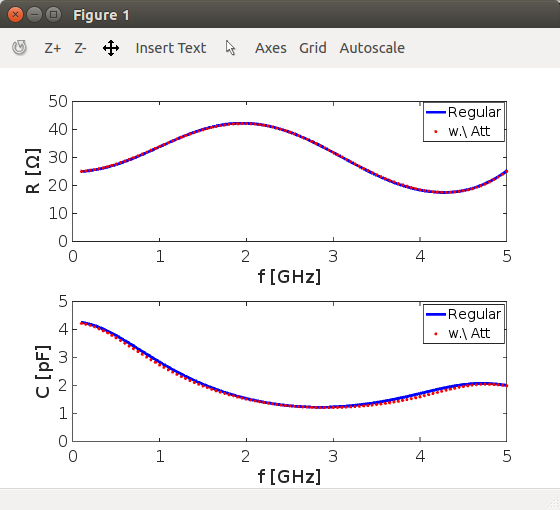
Well, it’s basically the same idea, but we filtered out extreme cases, so when the load impedance is significantly lower/higher, the results will at least be kept within physical boundaries.
Possible Improvements
A possible improvement would be to curve-fit or optimize the full de-embedding model, with the variable impedance transmission line. Such a feat will need to be done along all of the sampled frequencies, with some assumptions about the T-Line. This is a highly non-linear and transcendental equation, with 3 degrees of freedom. Hence Multi-variable optimization or curve-fitting is the way to go.
I have given this a go or two the past few weeks, but to no avail so far. Most of the work I have done was analytical attempts at the problem (approximating with several order, etc.), but maybe the brute-force method would have been better.
So that’s it. I have a lot more to say about de-embedding, with more complex and generalized models. For now I’ll take a break from this subject, but when I’ll get back to it, I’ll continue with 3 degrees of freedom, which is far more useful when you cannot make any assumptions about the de-embedded medium. Keep safe!