It occurred to me recently that although I named this site RF with care (for reasons I definitely cannot recall any more), I have not really written here anything RF or EM related in any way. So to start it off, why not start with my favourite: De-embedding.
1. What is De-Embedding anyway
If you already know what it is, feel free to skip to the next section. If not, then consider this: There is a good chance you are going to need to measure S-parameters. If you are already an RF engineer, this shouldn’t be a surprise to you. We all start a design with a simulation. However, while simulating your structure, you can place your ports basically anywhere. Even if you don’t really want a port, you can place a discrete, zero space consuming directional coupler, and you can calculation the parameters without any effect on the rest of the circuit.

However, let’s say that you can’t connect anywhere you like. Let’s say, as might be in a practical problem, that you can only connect at a certain distance from the Device Under Test (DUT) via a given connector. What you need to do here is to de-embed the unwanted portion, to measure in the correct reference plane.
2. 1st order problem explained
Fair is fair: All of the simulations presented here are performed with the wonderful QUCS. You can read my short review on it here. Be sure to check it out if you need some open source circuit simulation tools. If you need hard-core spice stuff, this still isn’t your tool, but for basic S-parameter simulation this is very good. The documentation and application notes there are terrific, and you can learn a lot from there about circuit simulator basics. Now, back to the problem. In this post we discuss only the case that a portion of transmission line separates between us and the desired reference plane. Meaning, there are two a-priori assumptions:
- The transition is of constant characteristic impedance (say, 50 Ohm). Yes, including the connector itself. Dealing with the connector is a different problem to be dealt with, in a 2nd order model at least.
- The line itself is of constant characteristic impedance.
This model is sometimes known as port extension (take a look at the network analyser near you) as it, in general, elongates the transmission line already calibrated.

3. How to model line
Well the good news are that a single transmission line is the easiest to model. The scattering matrix (S-parameters) for a lossless transmission line will look like this:
![\mathbf{S}_{TL} = \left[{\begin{matrix}0 & \mathrm{e}^{-j\theta} \\ \mathrm{e}^{-j\theta} & 0\end{matrix}}\right]\,;\,\,\theta = \beta l](https://s0.wp.com/latex.php?latex=%5Cmathbf%7BS%7D_%7BTL%7D+%3D+%5Cleft%5B%7B%5Cbegin%7Bmatrix%7D0+%26+%5Cmathrm%7Be%7D%5E%7B-j%5Ctheta%7D+%5C%5C+%5Cmathrm%7Be%7D%5E%7B-j%5Ctheta%7D+%26+0%5Cend%7Bmatrix%7D%7D%5Cright%5D%5C%2C%3B%5C%2C%5C%2C%5Ctheta+%3D+%5Cbeta+l&bg=ffffff&fg=000000&s=3 "\mathbf{S}_{TL} = \left[{\begin{matrix}0 & \mathrm{e}^{-j\theta} \\ \mathrm{e}^{-j\theta} & 0\end{matrix}}\right]\,;\,\,\theta = \beta l")
where beta is the propagation coefficient given in [1/m] and l is the length of the transmission line. The lossy matrix adds the loss coefficient, alpha:
![\mathbf{S}_{TL} = \left[{\begin{matrix}0 & \mathrm{e}^{-\gamma l} \ \mathrm{e}^{-\gamma l} & 0\end{matrix}}\right]\,;\,\,\theta = \beta l](https://s0.wp.com/latex.php?latex=%5Cmathbf%7BS%7D_%7BTL%7D+%3D+%5Cleft%5B%7B%5Cbegin%7Bmatrix%7D0+%26+%5Cmathrm%7Be%7D%5E%7B-%5Cgamma+l%7D+%5C+%5Cmathrm%7Be%7D%5E%7B-%5Cgamma+l%7D+%26+0%5Cend%7Bmatrix%7D%7D%5Cright%5D%5C%2C%3B%5C%2C%5C%2C%5Ctheta+%3D+%5Cbeta+l&bg=ffffff&fg=000000&s=3 "\mathbf{S}_{TL} = \left[{\begin{matrix}0 & \mathrm{e}^{-\gamma l} \ \mathrm{e}^{-\gamma l} & 0\end{matrix}}\right]\,;\,\,\theta = \beta l")
If you are not familiar with scattering matrices, please refer to Pozar’s Microwave engineering (or any other source, this is simply the best). Important: If you know the properties of the transmission line in the problem, it is possible to insert both alpha and beta into the equation as constants. If not, as will be shown in a moment, the result will be ambiguous and only return loss can be measured.
4. How to de-embed
The goal, if not defined previously, is to measure the “correct” return loss, in case of a one port network and to also de-embed the unwanted phase of a transmission measurement, in case of a two port network. Numbering the reference planes as such

we obtain the two following definitions

Substituting into the set of equations defined by the previous scattering matrixwe obtain

So while our measurement instrument measures the Return Loss (RL) in port #1, using the formula above we can obtain the RL in port #2. Notice that in this specific case, the phase is double. This is important while we discuss the ambiguity of the problem.
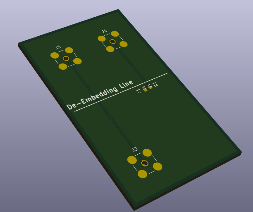
But in order to determine the S-parameters of the transmission line, we first need to measure them. For this, a common practice is a mirror or butterfly structure. Simply duplicate the structure, and connect it to each other. For example, here are two SMA ports connected by a transmission line of double length of what we will actually find in the circuit.
This way, when measuring double transmission line, the desired S-parameter matrix is obtained. Ideally, the primary diagonal is very close to zero, and the secondary diagonal represents double the distance travelled:
![\mathbf{S}_{Mirror} = \left[{\begin{matrix}0 & \mathrm{e}^{-2\gamma l} \\ \mathrm{e}^{-2\gamma l} & 0\end{matrix}}\right]](https://s0.wp.com/latex.php?latex=%5Cmathbf%7BS%7D_%7BMirror%7D+%3D+%5Cleft%5B%7B%5Cbegin%7Bmatrix%7D0+%26+%5Cmathrm%7Be%7D%5E%7B-2%5Cgamma+l%7D+%5C%5C+%5Cmathrm%7Be%7D%5E%7B-2%5Cgamma+l%7D+%26+0%5Cend%7Bmatrix%7D%7D%5Cright%5D&bg=ffffff&fg=000000&s=3 "\mathbf{S}_{Mirror} = \left[{\begin{matrix}0 & \mathrm{e}^{-2\gamma l} \\ \mathrm{e}^{-2\gamma l} & 0\end{matrix}}\right]")
This, if you recall correctly, gives the exact quantity required to de-embed.Non ideal cases will be discussed in another post. Now half the distance can be extracted by a square root. But alas! The square root function is ambiguous! This can be resolved in two ways:
- If you are only measuring the RL of one port, then it was already shown that the formula uses the square of the phase\loss found, and the ambiguity is resolved.
- If you are measuring a 2-port network and want the correct phase, then you must know the characteristics of the transmission line. This way the length, l, can be defined in a non-ambiguous way.
The popular way to define the de-embedding length is also the travel time in a known frequency, and is more commonly used in network analyzers.
5. Example
Hands on time! For this example, I will produce the S parameters of a double transmission line using QUCS.

The half matrix is produced using GNU Octave, with the script found in my GitHub.
De-embedding from the first reference plane to the desired one shows that the expected load is found correctly.
